Portfolio and Arbitrage

The mathematical theory of financial markets often begins with single-step discrete models that capture the fundamental ideas to build more complex models at both discrete and continuous time levels. It is also important to establish precise mathematical notations for familiar financial terms such as portfolio and arbitrage opportunity, which are essential for developing fair pricing or risk-neutral models.

In this chapter, we introduce the mathematical notions of portfolios, their values, and gains through which we establish a precise language for modelling market activities. We further give a general framework for building probability models that represent market uncertainty in a single time step that forms the foundation for more advanced multi-step models. An important concept explored in this chapter is arbitrage, which is a cornerstone of modern financial theory that ensures consistency in pricing and market equilibrium. As an application, we derive the forward pricing model and demonstrate how these concepts provide practical insights into real-world financial instruments.

Section «Click Here» establishes essential mathematical notations and defines, for a portfolio, its value and its gain. Additionally, this section illustrates the idea of constructing a probabilistic model for a finance market. Section «Click Here» introduces an important concept of derivative pricing, the arbitrage opportunity and its applications in developing forward and future pricing models.

Portfolio Concepts

We denote a collection of securities with deterministic cashflow (such as bonds and bank accounts) by

and a collection of risky securities (such as stocks) by

A capital market (also referred to as spot market or underlying market in the context of derivatives) is a collection of assets \(\big(\boldsymbol{B},\boldsymbol{S}\big)\).

A collection of derivative securities

is a derivatives market.

A market is a collection of securities \((\boldsymbol{B}, \boldsymbol{S},\boldsymbol{H})\).

Once a market is fixed, a portfolio can be defined as a mathematical representation of the quantities of different assets held in the market.

Value and Gain Processes

Once the portfolio is built, its value can be determined at every time instance.

Market Model

Let us start with a single step discrete capital market model which involves a probability space (\(\Omega, \mathcal{F}_*, \mathbb{P})\) on which the prices of the risky securities \(\boldsymbol{S}_1\) at time \(t_1\) are defined as non-negative random variables. Here, \(\Omega\) has a finite number of elements, \(\mathcal{F}_*\) denotes the power set of \(\Omega\) and \(\mathbb{P}\) is a suitably defined probability such that \(\mathbb{P}(\{\omega\}) > 0\), for all \(\omega\in \Omega\).

Obviously, at \(t_0=0\), we know the asset prices \(\boldsymbol{S}_0\), whereas the prices \(\boldsymbol{S}_1\) at \(t_1=T\) are unknown. Consequently, at time \(t=t_0\), a trader does not know the exact values of the asset prices \(\boldsymbol{S}_1\), but relies on the chosen probability model to quantify the uncertainty and study their potential behavior.

Predictable Strategy

Since a portfolio at a time is constructed based on the observed asset prices at that time, a collection of portfolios \(\Pi:=\{\Pi_k~|~k=1,2,\ldots\}\) can be viewed as a vector-valued stochastic process in \(\mathbb{R}^{n_b+n_s+n_h}\). For each \(k\), \(\Pi_k\) denotes the portfolio created at time \(t_{k-1}\) using the information available up to time \(t_{k-1},\) and held unchanged on the interval \([t_{k-1}, t_k).\) We refer to this portfolio process as a portfolio strategy or simply a strategy.

We are interested in predictable strategy.

Our next task is to specify a market filtration, which represents the information available to traders over time. In other words, we look for a filtration with respect to which the price process \(\boldsymbol{S}=\{\boldsymbol{S}_t\}\) is adapted (see Definition «Click Here» ).

For a given stochastic process \(\boldsymbol{S}\), we can always choose a filtration which makes the process adapted. Such a filtration, the natural filtration, is already illustrated in Example «Click Here» . We can also construct natural filtration through generated \(\sigma\)-fields from random vectors.

Our next question is the following:

Is every portfolio process a predictable process with respect to the natural filtration?

Self-financing Strategy

Another important condition that we impose on a trading strategy is the self-financing condition, which rules out any infusion or withdrawal of external capital during the trading period.

Next, we recall a result from basic probability theory, which is used in Problem «Click Here» to establish the measurability properties of trading strategies.

Arbitrage Opportunity

An arbitrage opportunity in a market refers to the existence of a portfolio that yields a non-negative payoff with no possibility of loss and a strictly positive payoff with positive probability.

Such opportunities often arise in a market due to the mispricing of similar securities traded in different segments of the market. For theoretical flexibility, one may also include the condition that the initial value of the portfolio is zero. The concept of arbitrage is fundamental to many financial pricing models and serves as a key principle in understanding market efficiency.

Arbitrage Portfolio

Let us now formalize the concept of arbitrage with a rigorous mathematical definition. We begin by defining an arbitrage portfolio, which refers to a portfolio held from time \(0\) to time \(T\). Later, we will extend this notion to arbitrage strategies in a dynamic trading framework.

The presence of arbitrage indicates inefficiencies in the market, as rational investors would take advantage of these opportunities until the discrepancies are eliminated. In our course, we always assume that the market is viable.

Observe that the arbitrage condition of a portfolio depends on the probability measure that we use. In the above example, we have not explicitly defined the probability measure to check the arbitrage condition because the situation is intuitively clear. However, in other scenarios, we may need to consider a suitable probability measure to verify arbitrage conditions.

Application: Forward Pricing

In this subsection, we derive a deterministic model for forward price in the simplest scenario where there are no additional costs associated with holding the underlying asset until maturity. Recall that the forward price is the delivery price the buyer has to pay to the writer to own the underlying asset at the expiration time \(t=T\), whereas no money is exchanged at the time \(t=0\) when the contract is initiated. We denote the delivery price of a contract with the expiration \(t=T\) by \(F(0,T)\). The forward price evolves in time due to ongoing trades in the forward market and fluctuations in the underlying asset price. The forward price in the market at any time \(t\in [0,T]\) is denoted by \(F(t,T)\). The return in a forward contract for the long position is defined as

We make two basic assumptions:

1. Frictionless Trade: We always neglect the cost associated with brokerage, taxes, and any other charges involved in maintaining the portfolio. Such a valuation is referred to as the frictionless valuation.
2. Ideal Bank: The prevailing interest rate in a risk-free investment is the same for both lending and borrowing. Such an instrument is referred to as an ideal bank. Further, we assume that this instrument can lend and borrow any amount of money.

The model suggested in Theorem «Click Here» give a fair value for a forward price given a prevailing interest rate scheme.

Law of One Price

The derivative pricing models we derive in later chapters rely on assuming the market is viable. There are at least two methods that we can use to derive these models:

1. Arbitrage Portfolio Approach: First, propose a fair price for the contract and then justify it by showing that any deviation of the proposed fair price can lead to the construction of an arbitrage portfolio contradicting the viable market assumption; and

2. Replicating Portfolio Approach: This method involves constructing a portfolio that generates the same payoff as the required instrument at a future time and then applying the law of one price.

The law of one price is a fundamental principle in economics and finance, which states that identical assets should be priced consistently across different markets in an efficient market scenario. We extend this economic principle to a portfolio and give a mathematical framework to it.

We now prove a sufficient condition for a pair of portfolios to satisfy the law of one price.

Arbitrage Strategy

Observe that Definition «Click Here» introduced the concept of arbitrage for a static portfolio. This can be extended to a arbitrage strategy to incorporate dynamic arbitrage.

Thus, a market is said to have arbitrage opportunity if there exists a self-financing strategy \(\Pi\) in the market such that all the conditions in Definition «Click Here» hold now for the value process of the strategy \(\Pi\).

The concept of the law of one price, discussed in Section «Click Here», can also be extended to self-financing strategies.

Application: Future Contracts

A future contract is a derivative instrument that falls under the category of noncontingent claims in financial markets. These contracts represent agreements to buy or sell an underlying asset at a predetermined price on a specified future date, just like how forward contracts function.

Commonly traded underlying assets in futures contracts include:

1. Commodities such as agricultural products (e.g., wheat, corn, soybeans), energy products (like crude oil, natural gas), and metals (like gold, silver);

2. Financial instruments such as stock indices, stocks and interest rates; and

3. Currencies.

Let us take the period of a future contract as the interval \([0,T]\), where \(t=0\) marks the moment at which the contract is traded (exchanged between the writer/seller and the holder/buyer) and \(t=T\) is the expiration time (the future market closing time on the expiration date).

A futures market quotes a price for the underlying asset at every trading time \( t\in [0,T],\) referred to as the future price or the delivery price or the settle price, denote by \(f(t,T)\). This price represents the value at which the underlying asset is delivered at the expiration time \(T\). The price of the same asset at the spot market is often different from the future price, called the spot price and is denoted by \(S(t)\). Understanding the relationship between the future price and the spot price is important and is the primary focus of this section.

The basic working mechanism of futures contracts is similar to forward contracts. However, there are a few key distinctions between them:

1. Futures contracts are traded on organized exchanges, whereas forwards are typically traded over-the-counter (OTC).

2. Exchanges settle futures contracts on a daily basis through a process called marking to market, which means that the value of the contract is adjusted daily based on current market prices. In contrast, forwards only have physical settlements on the expiration date, where the underlying asset is delivered or exchanged.

Marking to Market

In a futures market, marking to market (MTM) refers to the process of adjusting the value of a futures contract based on the current future price of the underlying asset. This adjustment occurs daily, typically at the end of each trading day. MTM plays a crucial role in managing counterparty risk by ensuring that losses are immediately covered, thus reducing the risk of default.

First, let's explore how the MTM process operates in an exchange market. Consider a partitioned \(\boldsymbol{t} = (t_0=0, t_1, \ldots, t_{n-1}, t_{n}=T)\) of the interval \([0,T]\), where each \(t_k\), for \(k=1,2,\ldots, n\), is the closing time of the market on the \(k^{\rm th}\) trading day of the future contract.

Maintenance of Margin: If the margin in one of the parties' accounts falls below a certain threshold (typically 50% to 75% of the initial margin deposit), the exchange notifies the respective party to replenish the margin account. The additional funds deposited, known as variation margin, play a crucial role in ensuring that the margin account maintains the minimum level required, referred to as maintenance margin. The exchange actively monitors margin levels and enforces margin requirements to promote market stability and integrity. Failure to meet the maintenance margin requirement results in the closure of the position by the next trading day.

Let us illustrate the marking to market process in the following example:

An illustration of marking to market process. The underlying asset is 250 shares of Reliance and the expiration date is 28-th December 2023. The contract is initiated on 1-st December 2023 at the rate of ₹ 2400 per share.

Example:

Consider two parties, Party-B (buyer) and Party-S (seller), who entered into a futures contract for the Reliance stock on the 1\(^{\rm st}\) of December 2023 with a delivery price of \(f(0,T)=2400\). The contract expires on the 28\(^{\rm th}\) of December 2023, and the number of shares in the contract is 250 (lot size). Party-B took a long position, while Party-S took a short position.

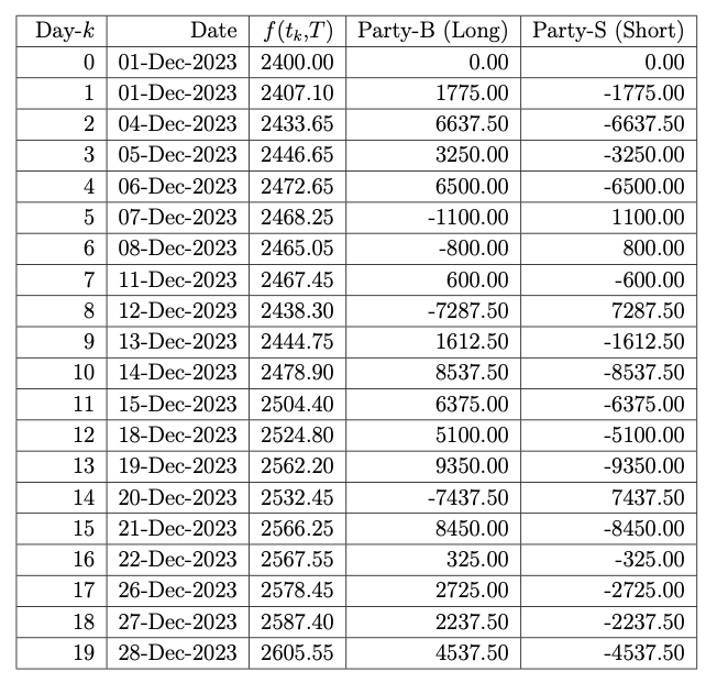
Assuming a margin requirement of 10% of the total trade value at expiry, the exchange requires an initial margin of ₹ 60000 from each party. The marking to market cash flows for Party-B and Party-S are shown in \tabl{marking.market.tb}, representing the daily adjustments in their margin accounts based on changes in the future price. We refer the table as the marking to market table.

Assume that a party gets maintenance margin call when the margin account goes below 50% of the requirement. Then, we see that the margin deposit of Party-S on 18\(^{\rm th}\) December evening had gone below 50% of the total margin requirement. Hence Party-S would have got a maintenance margin call from the exchange on this day to retain the position on the following day.

Problem:

A part of the Infosys stock's February future in the year 2021 is shown in the following table:

Assume that the futures contract is for 600 shares traded at a futures price of ₹ 1262.2 on the 1\(^{\rm st}\) of February. Construct the marking to market table and determine which of the two parties will face a maintenance margin requirement if 10% of the total delivery price is blocked as margin and 50% of the margin needs to be maintained.

Remark:

[Closing a contract]

The marking to market process continues in a contract until either the expiry date or one of the parties leaves the position by taking an equal and opposite position in the contract. For instance, if Party-B (long) wants to close the position in the contract before expiry, Party-B can enter into a contract of equal quantity (250 in the above example) where the position is a short position. This can be achieved by selling a contract of equal quantity of the same asset with an expiration date \(T\) in the future market. Similarly, if Party-S (short) wants to close the position, Party-S has to buy the same contract (with the same expiration date and asset) of equal quantity. Closing a contract is referred to as offset (or square off) the position.

Example:

Let us continue with the example from Example «Click Here» . If Party-B wants to off set the long position in the contract on December 8\(^{\rm th}\) (\(=t_6\)), then Party-B should sell a contract consisting of trading 250 shares of the same underlying asset with an expiration date of December 28, 2023. Whatever the delivery price of the contract at the time of selling will be considered as \(f(t_6,T)\) for the new short position of Party-B, and the marking to market process will be applied for that trading day. The total amount accumulated in the margin deposit will be finally paid back to Party-B by the exchange soon after the position is closed. Party-S's process will continue either until Party-S off sets the short position in a similar way or until the expiry.

Pricing Model

We now establish the futures pricing model assuming a constant prevailing interest rate throughout the futures contract period. We justify the model using replicating portfolio approach discussed in Section «Click Here». Since the basic mechanism of a future contract is the same as a forward contract, we construct two strategies, one with a forward contract and the other with an equivalent future contract, so that both lead to the same future value and are deterministic.

Recall that the future price \(f(t,T)\) (see Definition «Click Here» ) of the underlying asset generally differs from the spot price \(S(t)\). Similar to forward contracts, the future price \(f(t,T)\) tends to converge to \(S(T)\) as \(t \rightarrow T\), with \(f(T,T) = S(T)\).

Theorem:

Let the market allow long and short trades with fractional units and be a no-arbitrage market. If the prevailing interest rate remains constant throughout the entire period of the futures contract, then

\[ f(0,T) = F(0,T), \]

where \(T\) is the expiration time of the contract.

Proof:

Trades based on forward:

Construct a portfolio \(\Pi_F\) with the following trades:

1. Take a long forward position with forward price \(F(0,T)\) (no cost involved).
2. Invest \(e^{-rT}F(0,T)\) amount in a risk free asset.

We have \(\Pi_F = (1,0,1)\) and the initial value is

\[ V(\Pi_F)(0) = 1\times e^{-rT}F(0,T) + 1\times 0 = e^{-rT}F(0,T) . \]

At time \(T\), the value is

\[ V(\Pi_F)(T) = 1\times F(0,T) + 1\times (F(T,T) - F(0,T)) = S(T) . \]

Trades based on future:

For the sake of simplicity, we assume that marking to market is performed at just two intermediate time instances, \(0 < t_1 < t_2 < T\). Thus, we consider the partition \(\{t_0=0, t_1, t_2, t_3=T\}\) for the interval \([0, T]\). Note that in futures trading, each partition point \(t_k\) corresponds to a trading day, and therefore, the number of partitions should be equal to the number of trading days until the future expiration time. The argument below can readily be extended to cover more frequent marking to market.

At time \(t_0=0\): Construct a portfolio \(\Pi_{{f}_1}\) with the following trades:

1. Open a fraction of \(e^{-r(T-t_1)}\) units long in future (no cost involved).
2. Invest the amount \(e^{-rT}f(0,T)\) in a risk free interest rate investment (this investment will grow to \(f(0,T)\) at time \(T\)).

We have \(\Pi_{{f}_1} = (1,0,e^{-r(T-t_1)})\) with initial value

\[ V(\Pi^1_f)(0) = 1\times e^{-rT}f(0,T) + e^{-r(T-t_1)}\times 0 = e^{-rT}f(0,T). \]

At time \(t_1\): Make the following adjustments in \(\Pi_{{f}_1}\) to make a new portfolio \(\Pi_{{f}_2}\):

1. Receive (or pay) the amount \(e^{-r(T-t_1)}(f(t_1,T)-f(0,T))\) as a result of marking to market.
2. Invest (or borrow, depending on the sign) \(e^{-r(T-t_1)}(f(t_1,T)-f(0,T))\) in a risk free interest rate investment (this amount will be \(f(t_1,T)-f(0,T)\) at time \(T\)).
3. Increase the long futures position to \(e^{-r(T-t_2)}\) (no cost involved).

We have \(\Pi_{{f}_2}= \big((1,1), 0, e^{-r(T-t_2)}\big)\).

At time \(t_2\): Make the following adjustments in \(\Pi_{{f}_2}\) to make a new portfolio \(\Pi_{{f}_3}\):

1. Receive (or pay) the amount \(e^{-r(T-t_2)}(f(t_2,T)-f(t_1,T))\) as a result of marking to market.
2. Invest (or borrow, depending on the sign) \(e^{-r(T-t_2)}(f(t_2,T)-f(t_1,T))\) in a risk free interest rate investment (this amount will be \(f(t_2,T)-f(t_1,T)\) at time \(T\)).
3. Increase the long futures position to 1 unit (no cost involved).

We have \(\Pi_{{f}_3} = \big((1,1,1), 0, 1\big)\).

At time \(T\): The value of \(\Pi_{{f}_3}\) at \(t_3=T\) is

\begin{eqnarray} V(\Pi_{{f}_3})(T) &=& 1\times f(0,T) + 1\times (f(t_1,T)-f(0,T))+ 1\times (f(t_2,T)-f(t_1,T)) \\ &&~~~~~~~~~~~~+ (f(T,T)-f(t_2,T))\\ &=& S(T). \end{eqnarray}

(3.5)

Hence, the final wealth at maturity is \(S(T)\).

Observe that, the initial investment is \(e^{-rT}f(0,T)\) and the closing value is \(S(T)\). Thus, both the forward portfolio \(\Pi_F\) and the sequence of future portfolios \(\Pi_f:=\{\Pi_{{f}_k}: k = 1,2,3\}\) generate the wealth worth \(S(T)\) at time \(T\). Since, the market is assumed to be no-arbitrage, by Lemma «Click Here» , the law of one price holds for both \(\Pi_F\) and \(\Pi_f\). Hence, we have

\[ e^{-rT}F(0,T) = e^{-rT}f(0,T). \]

This completes the proof.

Remark:

The above theorem suggests that if the interest rate is constant, then the fair future price can be obtained using the formula

\[ f(t,T) = S(t)e^{r(T-t)}, \]

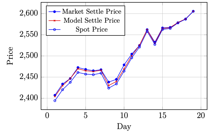
assuming that the underlying asset does not involve any extra costs or dividends. Deviation of futures prices from this model is typically attributed to anticipated changes in interest rates.

Example:

Although the interest rate is not constant in reality, the model proposed in Theorem «Click Here» \(~\) serves as an efficient predictor for routine analysis.

The figure below depicts the comparison of the market future price (settle price) with the model price obtained using the above formula with \(r=0.085\) and the spot price \(S\). The Reliance stock is used as the underlying asset in the depicted comparison result, where the future is for December 2023, spanning from the 1\(^{\text{st}}\) to the 28\(^{\text{th}}\) of December 2023 (also refer to Example «Click Here» ).

Reliance December 2023 future price comparison.

Problem:

Consider a future with 3 months expiry from today. Let the underlying asset be trading in the spot market at ₹ 1270. If the future price is currently trading at ₹ 1287.25, then find the corresponding prevailing interest rate.

Answer: \( r\approx 0.054\)

Remark:

There are three possibilities in the asset price movement, namely,

1. the asset price grows more than the prevailing interest rate;
2. the asset price grows, but less than the prevailing interest rate; and
3. the asset price decreases.

An investor takes a long position if the first case is predicted and takes a short position if one of the other two cases is predicted.

Project:

Write a python code that reads a csv file consisting of a monthly future data and makes another csv file with the following format:

Date, Settle Price, Model Price, Spot Price

Here, model price is obtained using the formula given in Remark «Click Here» , where \(r\) is taken as an input, whereas \(T\) is obtain by the code itself. Download the input csv file from the following link: NSE India Contract-wise Price Archives